
Statistics, Clergy Abuse, and Homosexuality: Coefficients
- YArespond
- Feb 7, 2019
- 4 min read

by Nathan
In the previous three posts, we gave an outline of Paul Sullins’ recent paper on homosexuality and clergy abuse. The first post gave a basic overview and discussed issues related to the data selected. The second post discussed correlation and the aggregation of data. The third post discussed polynomial transformation. This fourth and final post will discuss standardized coefficients and summary statistics.
Standardized Coefficients in Table 1
As mentioned in the previous post, the numbers in the first three rows of Table 1 in Sullins’ paper (E) are the standardized coefficients fit by the model. Standardized coefficients are analogous to the correlation coefficient explained above; they range from -1 to 1, respectively indicating perfect negative and perfect positive correlation.

The superscripts after the coefficients (*, **, ***) indicate the level of significance, measured by p-value. The levels can be found in the footnote (F). (P-value is a measure of the probability that the association between the predictors and the outcome variable quantified by the coefficients arose by chance; i.e. the probability that there is, in reality, no association at all.) The coefficients that don’t have a superscript following them are not statistically significant; that is, the probability that they arose by chance is too high for us to trust them. For example, because the percent of priests reporting a homosexual subculture lacks one of the symbols indicating significance in its the first three columns, we cannot conclude that its coefficient is different from zero. That is, we cannot truly determine correlation in that instance.

Check out this video for an explanation of P-values:
A final note about these coefficients: Sullins does not go in depth into what models he used or why he chose these particular ones to test his hypotheses. We should be curious why, for example, the coefficients for the models predicting percent male victims and abuse of males only are so different. Furthermore, as can be seen clearly from the table, the chosen predictors are often insignificant; in fact, the best predictor of percent male victims among the victims of multiple offenders is the (polynomially transformed) age at ordination variable. Finally, he provides no test of a null or alternative hypothesis, another item that is standard practice in research papers.
Summary Statistics in Table 1
Finally, the last three rows (Highest VIF, Model fit, R-square) are summary statistics concerning the quality of the model. VIF stands for variance inflation factor, which is a measure of our old friend multicollinearity (G). Sullins neglects to mention, however, that VIFs over 4 are generally taken to mean that some variables in the model may be collinear, which is the case for all but one of the models involving both variables under investigation. This means that the coefficients in these models cannot be trusted. We thus cannot trust any of Sullins’ model 2 coefficients, except for “Abuse incidents” which, according to the (high) 3.8 VIF, we should approach with skepticism. Because of these high VIF’s, these variables have a high chance of multicollinearity. (Roughly speaking, when multicollinearity is present, a model is more likely to calculate a p-value for a coefficient that is lower than what it should be. As a result we are more likely to conclude that a coefficient is different from 0 when in reality it may not be.)
Here’s a video on variance inflation factor. Just to warn you, it’s a bit technical…
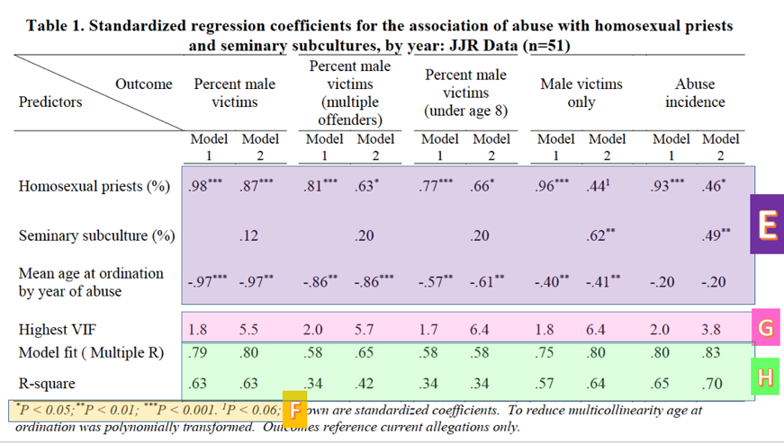
Sullins also includes the R-square for each model in Table 1. Multiple R and R-square are measures of model fit (H). Multiple R may be thought of as the correlation between the value predicted by the model and the actual value of the response variable for each set of observations, while R-square is a measure of how much of the variance in the outcome variable is explained by the predictor variables. Not only are these values much lower than the correlations reported earlier, they are much lower than is desirable for a quality model. I would not be comfortable presenting a model at my own work with an R-square less than .85 or so. Sullins’ range from .34 to .70.
Check out this video on R-squared, using house sales and work performance as examples:
Conclusion
In conclusion, not only are there questions about Sullins’ headline claims as they are presented; there are serious questions about his support of them. In the first place, measures of correlation are vulnerable to the phenomenon of spurious correlation and are sensitive to aggregation. We therefore cannot conclude without more support that the correlations Sullins reports are not spurious, particularly when they are measured on data that has been aggregated into five-year buckets. In the second place, the models Sullins builds in order to support these claims have several issues: These include an unexplained variable, potential multicollinearity, and lower numbers in general than those reported in his headline claims. Unless these issues are addressed, we cannot conclude to have learned anything new from the paper, which is highly susceptible to misleading representations. We should look elsewhere for empirical guidance.
Posts in this series:
4. Coefficients


Comments